BSCI 1510L Literature and Stats Guide: 5.4 A test for differences of sample means: 95% Confidence Intervals

In Section 5.3, we talked about differences and P-values in a general way.  Over the rest of this semester and next semester we will learn a number of particular statistical tests that are applicable to various types of experimental designs.  Each of those tests is designed to answer the same general question: "Are the differences I am seeing significant?" and each of those tests will attempt to answer that question by testing whether the value of P falls below the alpha level of 0.05 .  In order to answer this question, each of those tests will calculate the value of some statistical quantity (a "statistic") which can be examined to determine whether the value of P falls below 0.05 or not.  There are two approaches to making the determination.  One is to simply let a computer program calculate and spit out a value of P.  In that case, all that is required is to examine P and see if it falls below 0.05 .  The other approach is to specify a critical value for the statistic that would indicate whether P was less than 0.05 or not.  In this latter approach, the test does not produce an actual numeric value for P. 

This semester we will learn two commonly used tests for determining whether two sample means are significantly different.  The t-test of means (which we will learn about later) generates a value of P, while the test described in this section, 95% confidence intervals, allows us to know whether P < 0.05 without actually generating a value for P.

The concept of 95% confidence intervals is directly related to the ideas of sampling discussed in Section 3.2.2.  In that section we were interested in describing how close the means of samples of a certain size were likely to fall from the actual mean of the population.  The standard error of the mean (S.E.) describes the standard deviation of sample means of a certain sample size N.  In the example of that section, calculation of the S.E. allowed us to predict that 68% of the time when we sampled 16 people from the artificial Homo sapiens population, the sample mean would fall within 1.8 cm of the actual population mean.  32% of the time our sampling is less representative of the population distribution, and our sample means are more than one standard error from the true mean: more than 1.8 cm higher than the mean or more than 1.8 cm lower than the mean (i.e. outside of the range of 174.3 and 177.9 cm). 

Standard error of the mean is mathematically related to the probability of unrepresentative sampling.  4.5% of the time sample means would fall outside of the range of +/- two standard errors (172.5 to 179.7 cm).  0.3% of the time sample means would fall outside the range of +/- three standard errors (170.7 to 181.5 cm).  The wider the range around the actual mean, the less likely it is that sample means would fall outside it.  Since unrepresentative sampling is exactly what P-values assess, it is possible to define a range around a sample mean which can be used to assess whether that sample mean is significantly different from another sample mean.  This range is called the 95% confidence interval (or 95% CI).  The 95% CI is related to the standard error of the mean, and for large sample sizes its limits can be estimated from standard error:

Upper 95% confidence limit (CL) = sample mean + (1.96)(SE)

Lower 95% CL = sample mean – (1.96)(SE)

For smaller N, calculation of the 95% CI is more complex.  However, the 95% CI can be easily calculated by computer so we will simply use software to determine it.

If the 95% confidence intervals are known for two sample means, there is a simple test to determine whether those sample means are significantly different.  If the 95% CIs for the two sample means do not overlap, the means are significantly different at the P < 0.05 level.   

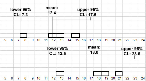
Fig. 9 Application of the 95% confidence interval test for the blood pressure drug trial with small sample size (old drug at top, new drug at bottom). 

Fig. 9 illustrates the situation described in Section 5.2 for the drug trial with very few test subjects (four per treatment).  Each white block represents one of the four test subjects.  In the figure, the sample means are shown as vertical lines, and the 95% confidence intervals are shown as error bars to the left and right of the vertical line.  If we apply the 95% confidence interval test to these results, we see that the difference between the sample means (5.4 mm Hg) cannot be shown to be significant because the upper 95% CL of the old drug exceeds the lower 95% CL of the new drug (the error bars overlap).  We would say that we have failed to reject the null hypothesis, i.e. failed to show that the response to the two drugs is different. 

Does that mean that there is actually no difference in the response to the two drugs?  Not really.  This is a really terrible drug trial because it has so few participants.  No real drug trial would have only four participants in treatment group.  The reality is that there is a great deal of uncertainty about our determination of the sample mean, as reflected in the relatively wide 95% confidence intervals.  It is quite possible that the response to the two drugs is actually different (i.e. the alternate hypothesis is true), and that if we improved our estimate of the mean by measuring more patients in our sample, the 95% confidence intervals would shrink to the point where they did not overlap.  On the other hand, it is also possible that the drug does nothing at all (the null hypothesis is true).   We may have just had bad luck in sampling and our few participants were not very representative of the population in general.  The only way we could have known which of these two possibilities were true would be if we had sampled more patients.  We will now examine how the situation could change under each of these two scenarios if we had more patients.

Fig. 10 Application of the 95% confidence interval test for the blood pressure drug trial with larger sample size (old drug at top, new drug at bottom) and alternative hypothesis true.

Let us imagine what would have happened under the first scenario (where the alternative hypothesis is true) if we had measured a total of 16 patients per group instead of 4.  Fig. 10 shows the first four measurement of each treatment as gray blocks and an additional 12 measurements as white blocks.  Because we have so many more measurements, the histogram looks a lot more like a bell-shaped curve.  In this scenario, the first four measurements were actually pretty representative of their populations, so the sample means did not change that much with the addition of 12 more patients.  But because with 16 samples we have a much clearer picture of the distribution of measurements in the sample, the 95% CIs have narrowed to the point where they do not overlap.  The increased sample size has allowed us to conclude that the difference between the sample means is significant.

Fig. 11 Application of the 95% confidence interval test for the blood pressure drug trial with larger sample size (old drug at top, new drug at bottom) and null hypothesis true.

Fig. 11 shows what could happen in the second scenario where the null hypothesis was true (the new drug had no different effect than the old drug).  Under this scenario, we can see that we really did have bad luck with our first four measurements.  By chance, one of the first four participants that we sampled in the old drug treatment had an uncharacteristically small response to the drug and the other three had a smaller response than the average of all sixteen patients.  By chance, three of the four participants who received the new drug had higher than average responses to the drug.  But now that we have sampled a greater number of participants, the difference between the two treatment groups has evaporated.  The uncharacteristic measurements have been canceled out by other measurements that vary in the opposite direction. 

Although the confidence interval is narrower with 16 participants than it was with four, that narrowing did not result in a significant difference because at the same time, the estimate of the mean for the two treatments got better as well.  Since under this scenario there was no difference between the two treatments, the better estimates for the sample means converged on the single population mean (about 16 mm Hg). 

In discussing these two scenarios, we supposed that we somehow knew which of the two hypotheses was true.  In reality, we never know this.  But if we have a sufficiently large sample size, we are in a better position to judge which hypothesis is best supported by the statistics.

By now you have hopefully gotten the picture that the major issue in experimental science is to be able to tell whether differences that we see are real or whether they are caused by chance non-representative sampling.  You have also seen that to a large extent our ability to detect real differences depends on the number of trials or measurements we make.  (Of course, if the differences we observe are not real, then no increase in sample size will be big enough to make the difference significant.) 

Our ability to detect real differences is called statistical power.  Obviously we would like to have the most statistical power possible.  There are several ways we can obtain greater statistical power.  One way is to increase the size of the effect by increasing the size of the experimental factor.  An example would be to try to produce a larger effect in a drug trial by increasing the dosage of the drug.  Another way is to reduce the amount of uncontrolled variation in the results.  For example, standardizing your method of data collection, reducing the number of different observers conducting the experiment, using less variable experimental subjects, and controlling the environment of the experiment as much as possible are all ways to reduce uncontrolled variability.  A third way of increasing statistical power is to change the design of the experiment in a way that allows you to conduct a more powerful test.  For example, having equal numbers of replicates in all of your treatments usually increases the power of the test.  Simplifying the design of the experiment may increase the power of the test.  Using a more appropriate test can also increase statistical power.  Finally, increasing the sample size (or number of replicates) nearly always increases the statistical power.  Obviously the practical economics of time and money place a limit on the number of replicates you can have.  

Theoretically, the outcome of an experiment should be equally interesting regardless of whether the outcome of an experiment shows a factor to have a significant effect or not.  As a practical matter, however, there are far more experiments published showing significant differences than studies showing factors to not be significant.  There is an important practical reason for this.  If an experiment shows differences that are significant, then we assume that is because the factor has a real effect.  However, if an experiment fails to show significant differences, this could be because the factor doesn't really have any effect.  But it could also be that the factor has an effect but the experiment just didn't have enough statistical power to detect it.  The latter possibility has less to do with the biology involved and more to do with the experimenter's possible failure at planning and experimental design - not something that a scientific journal is going to want to publish a paper about!  Generally, in order to publish experiments that do not have significant differences it is necessary to conduct a power test.  A power test is used to show that a test would have been capable of detecting differences of a certain size if those differences had existed.

Note: to calculate the descriptive statistical values in this section, you must have enabled the Data Analysis Tools in Excel.  This has already been done on the lab computers but if you are using a computer elsewhere, you may need to enable it.  Go to the Excel Reference homepage for instructions for PC and Mac.

To calculate the 95% CI for a column of data, click on the Data ribbon.  Click on Data Analysis in the Analysis section.  Select Descriptive Statistics, then click OK.  Click on the Input Range selection button, then select the range of cells for the column.  If there is a label for the column, click the "Labels in first row" checkbox and include it when you select the range of cells.  Check the Confidence Level for Mean: checkbox and make sure the level is set for 95%.  (You may also wish to check the Summary statistics checkbox as well if you want to calculate the mean value.)  To put the results on the same sheet as the column of numbers, click on the Output Range radio button then click on the selection button.  Click on the upper left cell of the area of the sheet where you would like for the results to go.  Then press OK.  The value given for Confidence Level is the amount that must be added to the mean to calculate the upper 95% confidence limit and that must be subtracted from the mean to calculate the lower 95% confidence limit.

Sickbert-Bennett et al. (2005) compared the effect of a large number of different anti-microbial agents on a bacterium and a virus.  They applied Serratia marcescens bacteria to the hands of their test subjects and measured the number of bacteria that they could extract from the hands with and without washing with the antimicrobial agent.  [The distributions of bacterial samples tend not to be normally distributed because there are relatively large numbers of samples with few bacteria, while a few samples have very high bacterial counts.  Taking the logarithm of the counts changes the shape of the distribution to one closer to the normal curve (see Leyden et al. 1991, Fig. 3 for an example) and allows the calculation of typical statistics to be valid.  Thus we see this kind of data transformation being used in all three of the papers.]

Fig. 12 Sample mean log reductions and 95% confidence intervals from Table 3 of Sickbert-Bennett et al. (2005)

For each type of agent, Sickbert-Bennett et al. (2005) calculated the mean decline in the log of the counts as well as the 95% confidence intervals for that mean (Fig. 12).  By examining this table, we can see whether any two cleansing agents produced significantly different declines.  For example, since our experiment will be focused on consumer soap containing triclosan, we would like to know if Sickbert-Bennett et al. (2005) found a difference in the effect of soap with 1% triclosan and the control nonantimicrobial soap.  After the first episode of handwashing, the mean log reduction of the triclosan soap was greater (1.90) than the mean log reduction of the plain soap (1.87).  However, the lower 95% confidence limit of the triclosan mean (1.50) was less than the upper 95% confidence limit of the control soap mean (2.19).  So the measured difference was not significant by the P<0.05 criterion. 

The method of checking for significance by looking for overlap in 95% confidence intervals has several weaknesses.  An obvious weakness is that the test does not produce a numeric measure of the degree of significance.  It simply indicates whether P is more or less than 0.05 .  Another is that it can be a more conservative test than necessary.  In an experiment with only two treatment groups, if 95% confidence intervals do not overlap, then it is clear that the two means are significantly different at the P<0.05 level. However, confidence intervals can actually overlap by a small amount and the difference still be significant. 

Another more subtle problem occurs when more than two groups are being compared.  The more groups that are being compared, the more possible pairwise comparisons there are that can be made between groups.  This increase in possible pairwise comparisons does not increase linearly with the number of groups.  If the alpha level for each comparison is left at 0.05, more than 5% of the groups whose means are the same will erroneously be considered to be different (i.e. the Type I error rate will be greater than 5%).  Thus a simple comparison of 95% confidence intervals cannot be made without adjustments.  In a scathing response, Paulson (2005) points out that Sickbert-Bennett et al. (2005) did not properly adjust their statistics to account for multiple comparisons.  According to Paulson, this mistake (Point 3 in his paper) along with several other statistical and procedural errors made their conclusions meaningless.  This paper, along with the response of Kampf and Kramer (2005) make interesting reading as they show how a paper can be publically excoriated for poor experimental design and statistical analysis. 

Despite these problems, 95% confidence intervals provide a convenient way to illustrate the certainty with which sample means are known, as shown in the following section.

Kampf, G. and A. Kramer. Efficacy of hand hygiene agents at short application times. American Journal of Infection Control 33:429-431.  http://dx.doi.org/10.1016/j.ajic.2005.03.013

Leyden J.J., K.J. McGinley, M.S. Kaminer, J. Bakel, S. Nishijima, M.J. Grove, G.L. Grove. 1991. Computerized image analysis of full-hand touch plates: a method for quantification of surface bacteria on hands and the effect of antimicrobial agents, Journal of Hospital Infection 18 (Supplement B):13-22.  http://dx.doi.org/10.1016/0195-6701(91)90258-A

Paulson, D.S. 2005. Response: comparative efficacy of hand hygiene agents.  American Journal of Infection Control 33:431-434.  http://dx.doi.org/10.1016/j.ajic.2005.03.013

Sickbert-Bennett, E.E., D.J. Weber, M.F. Gergen-Teague, M.D. Sobsey, G.P. Samsa, W.A. Rutala. 2005. Comparative efficacy of hand hygiene agents in the reduction of bacteria and viruses.  American Journal of Infection Control 33:67-77.  http://dx.doi.org/10.1016/j.ajic.2004.08.005