Figs. 7 and 8 again

Fig. 7 Illustration of hypothesis that the new drug lowers blood pressure more than the old drug (the "alternative hypothesis")
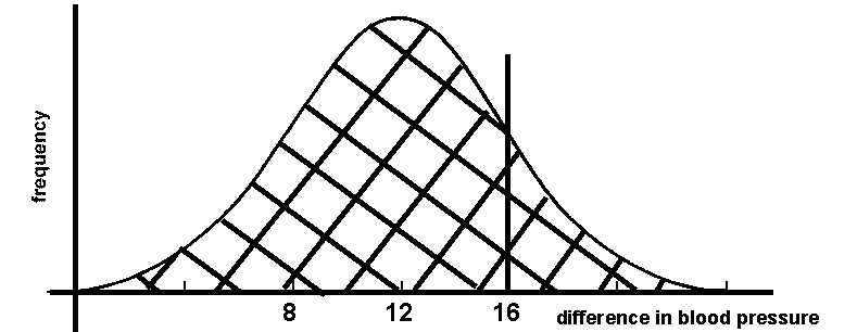
Fig. 8 Illustration of hypothesis that the new drug lowers blood pressure just as much as the old drug (the "null hypothesis")
5.2 P and Detecting Differences in Variable Quantities
In Section 4, we considered two possible explanations for the outcome of a blood pressure drug trial. One possibility was that the new drug affected blood pressure just the same as the old drug. This was illustrated in Fig. 8 where the two distribution curves of patient responses were identical. The technical term for this first model is the null hypothesis (i.e. there is no difference). Another possibility was that the new drug produced a greater effect in lowering blood pressure than the old drug. This second model was illustrated in Fig. 7 and is known as the alternative hypothesis (i.e. there is a difference).
Recall the discussion of sampling in Section 3. If we could sample all possible members of populations, we would know the true means of those populations. Determining which of the two models above is correct boils down to knowing whether the actual population means of the two groups are the same or whether they are different.
If the means are the same, then we accept the null hypothesis.
If the means are different, we reject the null hypothesis and accept the alternative hypothesis.
There are a variety of statistical methods that can be used to assess the likelihood that things are different or whether they are the same. In nearly every case, the outcome of the method is a quantity known as the P-value or just P. The P-value is an assessment of how likely the particular observed outcome would be to occur if the null hypothesis were true. If P is close to 1, then that particular outcome would be likely if there were no difference, while if P is close to 0, that particular outcome would be unlikely if there were no difference. In this description of P, the nature of what "different" means has been purposefully vague. Each kind of statistical test assesses a particular sort of difference, so the exact meaning of P varies with each test, but this general description applies to all tests.
In the example of Section 4, the difference we were assessing was whether the means of two populations were different - specifically whether the mean blood pressures of patients who received the new drug were different than the mean blood pressures of patients who received the old drug. The problem in Section 4.4 was that when we tested only a single patient who received the new drug, we had no way to assess whether that patient was typical of the drug-receiving population or not. In addition, Section 4.4 did not go into detail about how we would know how the responses to the old drug were distributed. In reality we would have to sample some patients who took the old drug to find that out.
Thus, to determine whether the drug has an effect or not, we would need to sample a number of patients who received the new drug and a number of patients who received the old drug. That would give us an idea of how the responses were distributed. We could then estimate the means of the two groups based on our samples and assess whether we thought the actual means were different or not. We know that sample means will never coincide exactly with the actual means so our assessment of whether the actual means are different will depend on how good we think the mean estimates are. Imagine that we collect some samples and determine that the sample means differ by a rather small amount of 5.4 mm Hg. How would we know how good our mean estimates were?
Recall the commuting example in the previous section. If we measured the length of the commute on only a few days (perhaps 3 or 4) out of the year, we might be unlucky and pick days when the commutes were not representative of typical commutes (unusually long or unusually short). On the other hand, if we measured the length of the commute on many days (perhaps 25), it would be very unlikely that we would happen to pick many days that were longer or shorter than usual. For each day we picked when the commute was longer than usual, we would probably pick another one that was shorter than usual to balance it out. So in general, the more commutes that we measure, the better our estimate will be and the less likely that our sample mean will be unrepresentative of the actual commute length.
Now consider the example where the sample mean of the new drug's effect is 5.4 mm Hg more than the old drug. Just like the variation in commutes, the intrinsic variation in the population response to the drug will tend to be random. If very few patients (e. g. four in each treatment) were sampled, there are two possibilities. One is that we got lucky and the few patients we tested were very representative of their populations. If that were true, then the 5.4 mm Hg difference in the sample means was a reflection of the real difference between the actual population means. However, if by chance one or several of the patients happened to have response that is unusually different from the actual mean for the treatment the patient received, it would have a big effect on the sample mean. If that were true, then the 5.4 mm Hg might have just been an artifact due to bad luck in sampling. If we conduct a statistical test, we might calculate a value of P=0.20 . What does that mean? When sample size is very small, it is fairly probable that the sample mean might differ a lot from the actual mean. If P=0.20, there is a 20% chance that we would get a difference of at least 5.4 mm Hg even if the new drug response is really the same as the response to the old drug. P could be considered an assessment of the probability of bad luck in sampling. Can we conclude that the measured difference in sample means of 5.4 mm Hg represents a significant difference? Most scientists would say "no" because even if there were no real difference (i.e. the null hypothesis; Fig. 8), one time out of five we would get a difference at least that big due to unrepresentative sampling.
If more samples were taken the outcome would become less uncertain. If by chance a particular patient were sampled who was more sensitive to blood pressure medications than average, it would be likely that you would test some other patient who was less sensitive. As you test more patients, their positive and negative deviations from the mean tend to cancel out and the sample mean tends to more closely reflect the true mean. The likelihood of getting a sample mean that is unrepresentative begins to fall. We begin to get a clearer picture of whether the distributions of the responses to the old and new drugs look like Fig. 7 or Fig. 8. If the actual distribution looks like Fig. 8 (i.e. the null hypothesis is correct), as more and more samples are taken (i.e. the sample size N increases), the difference between the sample means of the two drugs will approach zero and the value of P will rise toward 1. If the actual distribution looks like Fig. 7 (i.e. the alternative hypothesis is correct), there will continue to be a difference between the sample means (for illustration purposes let's say 6 mm Hg) and the value of P will fall. If we conduct a statistical test, we might calculate a value of P=0.001 . What does that mean? If P=0.001, there is a 0.1% chance that we would get a difference of at least 6 mm Hg even if the new drug response is really the same as the response to the old drug. Can we conclude that the measured difference in sample means of 6 mm Hg represents a significant difference? Most scientists would say "yes" because if there were no real difference (i.e. the null hypothesis; Fig. 8), we would only get a difference at least that big due to unrepresentative sampling one time out of a thousand. It is possible that we just had bad luck in sampling, but the probability is so low that we would reject the null hypothesis.
