BSCI 1510L Literature and Stats Guide: 3.2 Samples Versus Populations

In addition to the technical and mathematical components of experimental science there is also a major economic component.  If the quantity we want to study is the mass of all laboratory mice on earth, it is clear that we have neither the time nor money to measure all members of that population.  So an important question in nearly every experiment is "how many replicates should I measure" (or how many trials should I conduct, etc.).  More is almost always better, but how many is enough?  There is no simple answer to this question, but an understanding of the phenomenon of sampling and the statistics associated with it is a first step toward developing skill in designing successful experiments. 

The term population describes all of the possible members of a group (or outcomes of a particular treatment, etc.).  Often our goal is to know the mean of a population, but this is almost never possible because there are usually too many individuals to measure.  Instead, we depend on measuring samples that are a subset of the population.  When we calculate the mean of our sample, we hope and assume that it is similar to the population mean (also known as the parametric mean).  However, the extent to which that is true depends on which individuals we sample. 

If we happen to sample individuals that by chance are mostly smaller than the population mean, then our sample mean will be smaller than the population mean and vice versa.  The more variable the individuals are in a population, the more likely it is that we are going to sample individuals that deviate far from the mean (e.g. we are much more likely to sample a 15g mouse from the wild population than from the lab population).  If we sample multiple random individuals, we are just as likely to measure individuals that are larger than the mean than individuals that are smaller than the mean.  Thus, with more sampled individuals, the deviations from the population mean tend to cancel out and the resulting sample mean is expected to be closer to the true mean than with fewer samples. 

You can observe this phenomena in the Witlock and Schluter kingfisher sampling simulation mentioned at the top of this page.  To make the population more or less variable, slide the sigma slider further to the right or left and see how the means for many samples change.  To sample more or fewer individuals, slide the "n" slider further to the right or left and see how the means for many samples change. 

The following illustration involves heights of a population of 100 humans (Homo sapiens).  Since this is an artificial example, we are in the atypical position of being omniscient and knowing that the true mean height of the population is 176.09 cm (about 5 ft. 9 in.).  The standard deviation is 7.20 cm (about 3 in.), so about 2/3 of the individuals range from 168.89 cm to 183.29 cm (5 ft. 6 in. to 6 ft.).  The tallest individual in the population is 192.8 cm (6 ft. 6 in.) and the shortest is 160.0 cm (5 ft. 3 in.).  Fig. 3 shows a histogram of the population. 

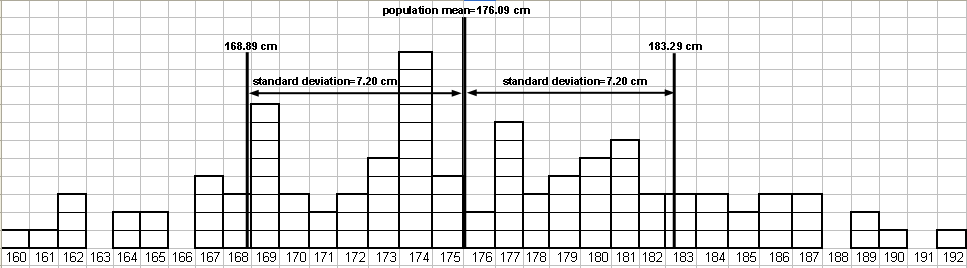
Fig. 3 Distribution of heights of 100 Homo sapiens individuals

Because of limited time and resources, some scientists (not omniscient!) are only able to randomly sample and measure 16 of the individuals. 

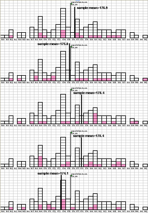
Fig. 4 Five samples of 16 from the H. sapiens population of Fig. 3, and their means

The individuals that they sample are shown as the shaded blocks in the first histogram at the top of Fig. 4.  They calculate a sample mean of 176.9 cm, which is pretty close to the true mean but a bit on the high side.  As we are enjoying our godlike status as the creators of this simulation, we exert our omnipotence and make time run backwards so that we can see what happens if the scientists conduct their experiment again.  The second time, they get lucky in their sampling and calculate a mean of 175.8 cm - remarkably close to the true mean!  Even though they happened to sample the tallest individual in the population, they sampled several of the shorter members, which canceled out the large deviation from the mean.  On the 3^rd through 5^th tries, the scientists aren't so lucky and they calculate sample means that are too high (tries 3 and 4) or too low (try 5) because by chance they sampled individuals that were less representative of the population than in the first two tries.

We now tire of the novelty of controlling an artificial universe and devote ourselves to the more practical task of answering the following question: is there a way to predict how close sample means will be to the true mean if we measure a certain number of samples?  Based on our experiment on the scientists, we can assess the variability in sample means by taking the standard deviation of the 5 means that the scientists collected.  The resulting standard deviation of those means is 1.82 cm.  The standard deviation of many means, each resulting from a certain number of samples, is given the special name: the standard error of the mean (or S.E.).

What does this number mean?  It means that if someone measures samples of 16 from our population of humans, about 2/3 of the time their sample mean will be within 1.82 cm of the true mean.  That is useful information, but only in our particular situation.  It would be better to have a more general way to predict how close sample means are likely to be to the true mean for any population.  The method of prediction would need to consider the standard deviation of the population because a more variable population would make it more likely that atypical individuals would be sampled.  It would also need to consider the sample size, because the more samples that are included, the more likely atypical individuals would be to have their deviation cancelled out by another individual that is atypical in the other direction.

It is possible to estimate the standard error of means derived from a certain number of samples (without actually sampling a lot of means and finding their standard deviation) by using the formula:

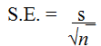                                                                                  Equation 4

where s is the standard deviation of the samples values and n is the number of samples (or sample size).  If we apply Equation 4 to our human population, which has a standard deviation of 7.20 cm, we find that with a sample size of 16 the standard error is estimated to be 1.80 cm.  This is quite close to the standard deviation that we actually calculated from the 5 sample means determined by our scientists. 

One problem with Equation 4 is that in order to calculate the standard error, we need to know the standard deviation of the population.  Since in real life we are mere mortals and don't know the true standard deviation of a population, we have to estimate the standard error using an estimate of the standard deviation that we calculate from our samples.  As was the case with the mean estimates made from samples taken by the scientists in the example, our estimates of the population standard deviation may vary from the true standard deviation if we are unlucky and sample individuals that aren't typical for the population.  This will cause our estimate of the standard error to vary from its true value as well.

There is a tendency on the part of students to confuse standard deviation and standard error of the mean (because they both have the word "standard" in their name??).  But it is important to be clear about the nature and use of these two statistics.  Standard deviation describes the variability of individuals in the population itself.  Standard error describes how much sample means are likely to vary from the true mean. In the Witlock and Schluter kingfisher sampling simulation, the distribution of the population can be shown by clicking on the "Show Population" button.  Click on that button, then slide the sigma slider back and forth to see how the population changes when the standard deviation changes.  The distribution of sample means can be shown by clicking on the "Show Sampling Distribution" button.  Click on that button and slide the three sliders (n, mu, and sigma) to see how they affect the standard error, which is represented by the width of the sampling distribution. 

In reporting the results of an experiment, you are likely to see either of these statistics, and often both.  Standard deviation is given if experimenters want to give an indication of the spread of the data they have collected.  Standard error is given if they want to indicate the level of confidence that they have in their estimate of the mean.