BSCI 1510L Literature and Stats Guide: 4 Variation and differences

In the Section 3 we examined how individuals varied within a population and how common statistical quantities describe that variation.  In this section we will examine how variation within a population affects our ability to detect differences.

For many years, we conducted an experiment involving determining whether genetic traits are linked on fruit fly chromosomes.  As a part of this analysis, we tried to measure whether crossing over in one part of the chromosome interferes with crossing over in another part.  If there is no crossing over, a coefficient of zero results and if there is crossing over, the coefficient is greater than one.  When we actually did the experiment, about half of the sections produced a coefficient of less than zero, which at first glance seemed to be an impossibility.  Invariably, this produced an army of students who marched to my office concerned about the fact that they didn't get the "right answer" and wondering what they did wrong.  It has been interesting to discuss the situation with the students because it has helped me to understand how most college freshmen and sophomores think about laboratory exercises.  Here is the general logic used by most students:

1.  There is a right answer to this problem.  The teacher knows it and my job is to find out what it is.

2. Because this question asks about crossover interference, there must be crossover interference, because otherwise, why would we be doing the lab?

3. My answer is negative, which is impossible to achieve because the lowest possible answer is zero.

4. Therefore I have messed up and must be making a big mistake somewhere.  I need to find out what I did wrong, otherwise I will get a bad grade and will never make it into medical school.

Before discussing the fruit fly experiment with the students, I ask them the following question:  If you have a family of four, how many boys and how many girls should you get?  Invariably the students can give the "answer": you should get 2 boys and 2 girls.  I tell them that my wife has three sisters and no brothers, then ask the students: what mistake was made by my wife's parents to produce four girls?  Most students have no trouble telling me that although the number of girls in a family having four children should average two, due to chance the number commonly varies above and below that number.  A quick glance at the fruit fly chromosome map shows that the gene loci we were considering are so far apart that it is unreasonable to expect that there should be any crossover interference and that we should expect that the calculated coefficient would be zero on average.  The puzzling negative number didn't mean that the students made a mistake.  The flies didn't make a mistake either!  We are simply observing small random variation around zero due to the unpredictable nature of sampling real flies, and sometimes that random variation results in a value slightly below zero. 

How does it happen that nearly all of the smart, capable, and motivated Vanderbilt undergrads in my class draw the incorrect conclusion in this circumstance?   As the parent of a high school student, I can see that the problem starts in about seventh grade.  In elementary school, children may be encouraged to observe and draw conclusions in a low-stakes environment.  But as high school approaches, the pressure builds to get good grades and high test scores.  In response, students become experts at figuring out what their teachers want and how to produce answers that are "right".  They have few experiences dealing with situations where the answer is not known, or where it is impossible to be certain that an answer is correct.  The situation is exacerbated by experiences in chemistry and physics classes, where matter is very well behaved and advanced measuring technology allows some physical characteristics to be measured accurately to 4 or more significant digits.  They come to expect that we can, and should, be able to produce "the answer" with a high degree of precision. 

These experiences put students on a collision course with real-world biology.  In real-world biology, there are a lot of things we don't know.  Because living organisms and systems are a lot more variable and a lot less well behaved than the simpler materials studied in chemistry and physics, there is uncertainty in most everything we work with.  So one of our major goals in this course is to help students get over their discomfort with uncertainty, and to give them the tools to quantify variability and make decisions in uncertain situations.  One of the first steps in this direction is to understand why results vary.

Imagine that you are a biomedical researcher and you are investigating a new form of a high blood pressure drug that is being developed by your company.  According to the published literature, the previous form of the drug lowered blood pressure by 12 mm Hg.  You administer your new version of the drug to a patient and find that it lowered the patient's blood pressure by 16 mm Hg.  You begin to imagine yourself in Stockholm accepting your Nobel Prize in medicine. 

Not so fast!  How do you know that your new version really lowers a patient's blood pressure 4 mm Hg below the current drug?  There are three possible reasons why your patient's blood pressure decrease is different from the decrease caused by the current drug (actually there is a fourth reason - the value published in the literature could be wrong, but for our purposes we will assume that value is correct):

4.2.1 Experimental error.  There could be something about the way that the experiment is being conducted that is causing you to mismeasure the true effect of the drug.  For example, the blood pressure cuff you are using to measure the patient may be out of calibration and is systematically skewing the measurements by a certain amount.  A machine used to manufacture the drug may have a loose bolt and be randomly adding larger or smaller amounts of the drug to the filler used to deliver the drug.  Your technician may be careless and not bother to measure the dose carefully.  This source of variation is the one most likely to be blamed by students for unexpected results, but if careful attention is paid to quality control and standardizing the experimental protocol, it is actually probably the smallest contributor to variation in results.

4.2.2 Intrinsic variation.  Patients are humans and humans are by their nature variable.  There are many uncontrollable aspects of a subject's life that could affect his or her response to a drug, including what they had for breakfast, whether they were suffering from an illness, and their general health at that time in their life.  If the very same dose of drug were given to the very same patient on another day, it is unlikely that the exact same decline in blood pressure would occur.  You would have a better idea of the drug's affect if you repeated the test on the same subject on several different days, but even so you would only be measuring the effect on that particular person.  In a drug test, we are more interested in the effect of the drug on people in general.  Because of differences in genetics and the particular environment in which people live, we expect that the different people will have different responses to a drug, so we need to test many different subjects before we can generalize our conclusions. 

4.2.3 Experimental effect.  This is the source of variation in which we are actually interested.  It is the amount that the blood pressure decline is changed by the effect of the new version of the drug.  If the effect of the new drug is small, it will be hard to notice in comparison to the variability among patients receiving the drug.  So we would like to make the experimental effect as large as possible.  One possible strategy would be to increase the effect by increasing the dose of the drug.  However, that could also have the undesired effect of killing the patient!

In any given situation, the actual variation in a particular result may be a combination of all three of the sources of variation described above.  For example, of the 4 mm Hg difference between the response of your patient to the new drug and the response of patients in general to the old drug, 1 mm Hg might be due to technician error in reading the blood pressure, 2 mm Hg might be because your particular patient responds to blood pressure drugs more sensitively than the general public, and 1 mg Hg might be due to the new drug's increased effectiveness over the old drug.  In that scenario, the effect of the drug would probably be so small that its development is a waste of time.  On the other hand, your technician might be really good and read the scale exactly, your patient might be having a response 9 mm Hg less than the general public because he is actually less sensitive to blood pressure medication than average, meaning that for an average person the new drug would actually lower blood pressure by 13 mm Hg more than the old drug.  In that case, the new drug would be a great improvement over the old one.  Another possibility is that there is actually no difference between the new drug and the old drug and that all of the variability is due to experimental error and intrinsic variation. 

To understand the possibilities better, we need to consider this one particular result in the context of all possible results.  In many situations, if we measure a large number of individuals and plot the frequency of each measured value (i.e. the number of times that we got that value) versus the magnitude of the value, a curve similar to the one shown below usually results.  This shape of curve is called the standard curve (also known as the "bell-shaped curve").

Fig. 5 Variation in population response to an experimental treatment

The peak of the standard curve is located at the mean (average) value for the population.  In the specific case of the drug test example, the peak of the curve could represent the average decrease in blood pressure as a response to the old drug for people in general.  Individuals in the population differ in many kinds of little ways, and each of these ways can cause their response to be shifted slightly higher or lower.  In many cases, small differences that shift the response higher are greater than the small differences that shift the response lower.  So there are quite a few people who have responses a little greater than average.  In relatively few cases, by chance individuals experience a lot of small differences that shift their response higher and experience only a few differences that shift their response lower.  So there are only a few people with responses a lot higher than average.  The same corresponding situation holds for situations where there are more small differences that shift the response lower than higher.  Thus the curve is symmetric with "tails" that get smaller at values further from the mean. 

Fig. 6  Variation in population response under more carefully controlled conditions

Although it is impossible to eliminate all variability in a population, we can reduce it if we carefully control the conditions of our experiment.  For example, if we limit the subjects of the experiment to women between the ages of 20 and 30, have them eat a standardized diet during the 24 hours before the experiment, and measure all their blood pressure changes at the same time of day, we may be able to eliminate a lot of the small differences among subjects that contribute to the variability and narrow the standard curve as shown in Fig.6.  Using the terminology from last week, we can say that we have reduced the standard deviation of the population. 

Let's return to the example of our blood pressure drug trial.  For the time being, let's assume that the new version of the blood pressure drug actually lowers blood pressure a lot more than the old drug.  This scenario is illustrated in Fig. 7.  The curve at the left represents the response of the test subjects to the old drug.  The average response of subjects to the old drug was 12 mm Hg, but you can see that many participants had responses as low as 8 and as high as 16.  The response of the same group of test subjects to the new drug is illustrated by the curve on the right.  The average response to the new drug is a lot higher (about 25 mm Hg).  The vertical line represents the bresponse of our one test subject whose blood pressure was lowered by 16 mm Hg.  You can see that under this scenario, by chance we were unlucky and picked a test subject who was less responsive to the new drug than normal. 

Fig. 7  Illustration of hypothesis that the new drug lowers blood pressure more than the old drug (the "alternative hypothesis")

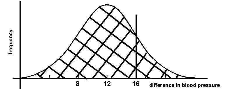
Fig. 8  Illustration of hypothesis that the new drug lowers blood pressure just as much as the old drug (the "null hypothesis")

Fig. 8 shows another possible scenario.  In this scenario, the new version of the blood pressure drug is a failure because it doesn't work any better than the old version.  Test subjects respond exactly the same to the new drug as they do to the old drug and the normal curves representing the two drug responses are exactly on top of each other.  Under this scenario, our one test subject whose blood pressure was lowered by 16 mm Hg was actually more responsive to the drug than average. 

So which of these two hypotheses is correct?  With a single test subject there is absolutely no way that we can have any idea whether one hypothesis is supported more than the other.  In order to know whether the response curve of subjects to the new drug is different than the response curve to the old curve, we will need to test enough people to determine the actual shape of the curve. 

Let's return to our original discussion of the causes of variability to see how they are related to the figures above.  If the experimental error has a random effect (such as sloppiness in measuring or the loose bolt), then it contributes to a larger standard deviation (i.e. Fig. 5 vs. Fig. 6) of the response curves.  Random experimental error can be reduced by carefully controlling the conditions under which the experiment is conducted.  The result would be a decrease in the area of overlap in Fig. 7, which would make it easier to tell whether the two curves were different.  If an experimental error was systematic (as in the example of the badly calibrated pressure cuff), then the result might be a shifting of the entire curve to the left or right.  This would be very bad if only one or the other of the curves was shifted because one would think that the two curves were either more or less different than they really were.  On the other hand if the same miscalibrated cuff were used to measure both groups, then they might be both shifted the same amount.  That would be less problematic because the difference between the two groups would still be the same even if the actual pressure readings were incorrect. 

As we have already discussed, we can reduce the intrinsic variability of our experimental population by controlling or eliminating factors that influence our subjects' response, but which are unrelated to the factor that we are studying.  For example, white laboratory mice are preferable to wild mice as test subjects in drug trials because the white mice have experienced nearly identical environmental conditions and are genetically very similar.  With reference to Fig. 7, white lab mice would have very narrow curves (small standard deviations) and the curves could be relatively close together without having a very large area of overlap. 

Finally, the experimental effect is represented by the difference between the peaks of the two response curves.  The experimental effect can range from zero (if the null hypothesis is correct and the treatment has no effect) to larger values (if the alternative hypothesis is correct and the treatment has an effect).  If there is a non-zero experimental effect, it can sometimes be made greater by increasing the intensity of the treatment.  This would result in a greater separation between the peaks in Fig. 7 and a decreased area of overlap. However, there are usually limits to the intensity of the treatment since more intense treatments may result in death or damage to the experimental subjects. 

Clearly coming up with a strategy for differentiating among the different sources of variability is important for an experimental scientist.  The subject of controlling experimental conditions so that unwanted variability is reduced and experimental effects are increased is called experimental design and will be a major focus of this course.  The mathematical tools for measuring and assessing variation (statistics) are also very important and we will develop skills in using them over the next several weeks.