BSCI 1510L Literature and Stats Guide: 1 Formulas in Excel

When you type something in a cell in Excel, it decides what kind of thing you are putting there by the characters you type.  If you type a number, it guesses that you intend a number.  If you type letters, it guesses you intend text.  To tell Excel that you intend a cell to contain a formula rather than text or numbers, the contents of the cell must start with an equals ( = ) sign. 

Although you can create a formula that simply performs numeric operations on numbers, that is usually pointless because you could just do such calculations with a calculator.  The real power in Excel comes from its ability to repeat the same kind of calculation on many cells in a spreadsheet.  To make a calculation generic enough to repeat it for many cells, one must create a formula that uses cell references.  Each cell is referenced by its column letter and row number, e.g. B3.  If you are creating a formula, Excel assumes that anything that you type which consists of a letter followed by an integer number (or several letters followed by an integer number) will be a cell reference. 

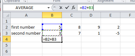
To create a formula in a particular cell, click on the cell where you want the formula to go.  Type an equals sign and then start putting in cell references.  When constructing a formula, it is often easier to let Excel enter the cell reference by clicking on the cell to which you want to refer.  You can insert mathematical operators between cell references by pressing the appropriate key (+, -, *, /, ^, and parentheses).  To terminate the entry of the formula, press the enter key.  The following example illustrates this.

If you copy and paste a formula into another cell, Excel is really clever.  It assumes that you would like whatever relationship you have expressed among cells to be continued, but shifted in the direction of the cell into which you've pasted the formula.  In the example above, if you copy the contents of cell B4 into cell D4 (two columns to the right), the formula in D4 will add cells D2 and D3 (which are two columns to the right of B2 and B3) and calculate a value of 10.  If you copy the formula from B4 into B5 (one row down), the formula in B5 will add cells B3 and B4 and calculate a value of 11. 

When a cell is selected, the lower right corner will have a small square on it.  Mousing over that square will cause the cursor to become a black cross.  If one clicks and drags the small black square with the black cross, Excel will effectively copy and paste the formula from the selected cell into every cell that the cursor is dragged across.  (In some older versions of Excel, there is a slight difference in the behavior of the fill handle compared with copy and paste.  If the fill handle of a cell containing a number is dragged, Excel increments the number by one.  However, this does not happen in newer versions of Excel.)  If a row of cells is selected and the fill handle in the lower right corner of the selection is dragged down, every formula in the row will be copied to the cell below with the cell references changed to the next row down.  Selecting a column of cells and dragging its fill handle to the right or left, or dragging the fill handle of a row of cells up have similar behaviors relative to their respective directions. 

Sometimes one wants the reference to a cell to remain constant.  In the following example:

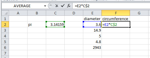
we would like for each value in the E column to be multiplied by pi in the formula in the F column when we paste the formula from cell F2 into cells F3 to F6.  However, if we use a regular cell reference to C2, then the formula would increment the second cell reference in the formula and multiply each diameter by the blank cells below cell C2.  To prevent Excel from changing the number part of the cell reference (i.e. to hold the row constant), put a dollar sign ( $ ) before the number part.  To prevent Excel from changing the letter part of a cell reference (i.e. to hold the column constant), put a dollar sign in front of the letter part.  To always refer to one particular cell no matter where a formula is pasted, put dollar signs in front of both the number and letter part (e.g. $C$2 ).

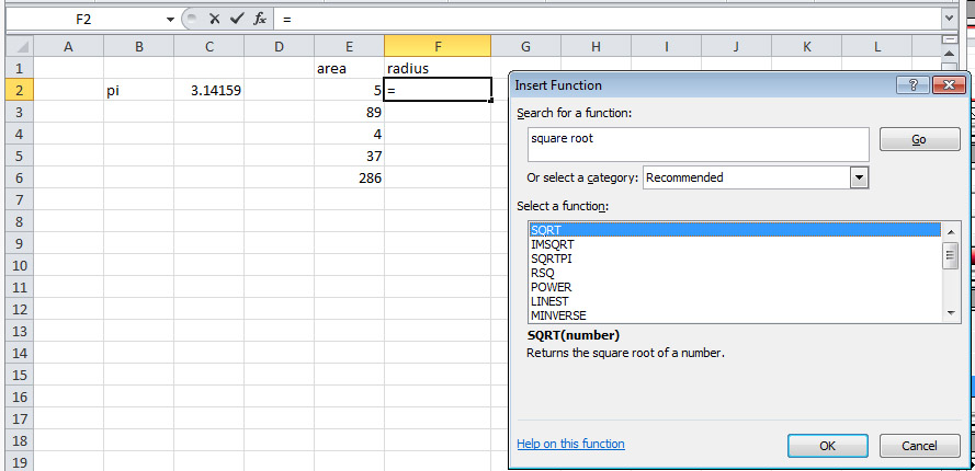
In addition to the simple math operators (e.g. +, -, etc.) Excel has many built-in functions for performing more complicated operations.  One can make use of these functions by typing them into a formula (i.e. a cell whose contents begin with "=") but it is easier to select them from a list.  To insert a function in a formula (or blank cell), click on the little f_x symbol to the left of the character entry box.  This will bring up a dialog box that you can use to select the formula you want:

After you have selected a function, it will be inserted into the formula in the character entry box.  Another dialog box will come up for you to enter the formula arguments.

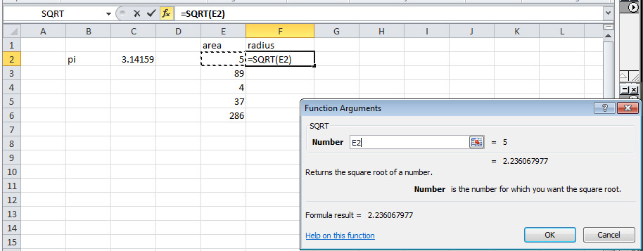
In the example above, the square root function operates on a single number.  So a single cell reference should be entered in the Number box.  Alternatively, you can click on the cell and Excel will enter the reference to that cell in the box for you.  If the cell you want to click on is hidden by the dialog box, click on the "hide dialog box" button:

to reveal the cells underneath.  Click OK and then continue editing the function until you are done.

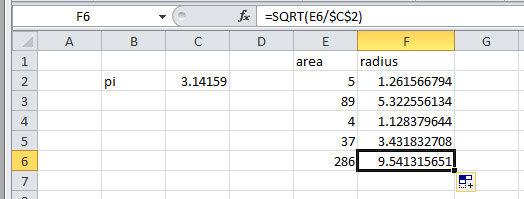
The figure above shows the completed formula.  The argument of the square root function was modified to divide by pi by clicking after the E2 cell reference in the character entry box and typing "/$C$2".  The formula was then copied into the cells below.  When editing a formula in the character entry box (i.e. the cursor is in that box), one can enter cell references by clicking on cells, or change cell references by highlighting an existing cell reference and then clicking on the new cell.  Excel will color code the cell references with the cells to make it easier to see where the arguments of the formula are coming from.

In some cases, the function has arguments which are a range of cells rather than a single cell.  In that case, the beginning and ending cell references separated by a colon are entered as a function argument.  For example, the formula

=MAX(F2:F6)

will produce the largest value in cells F2 through F6.  As was the case with a single cell, during the argument entry phase, the range of cells can be selected by clicking and dragging across the range of cells on the spreadsheet and Excel will fill in the appropriate cell range.